ShinyCFA App

Note: ShinyCFA is not currently being actively maintained but is still hosted at https://nickrongkp.shinyapps.io/ShinyCFA/. The application takes a while to load but is cheaper than AWS.

Motivation

ShinyCFA was developed with Nick Rong while learning to build R Shiny applications. We both had an interest in producing interactive applications that could be used to support our work and this was built with that goal in mind. The project was mainly completed in late 2019 but was recently used as a test application to deploy a Shiny app on both AWS and shinyapps.io. However, to reduce fees and maintenance it is currently only hosted on shinyapps.io and can be accessed at: https://nickrongkp.shinyapps.io/ShinyCFA/

The code is also available on github.

Application Overview

The purpose of the application is to allow a water resource practitioner to easily access, explore, and conduct preliminary analyses using streamflow data available from the Water Survey of Canada (WSC). Archived WSC streamflow data are stored in the HYDAT database which is available in a SQLite format.

The ability for the application to search and extract data from the HYDAT database is provided by the tidyhdat package which is maintained by the British Columbia government. Accordingly, much of the data access functionality of the app can easily be done directly within R, but the app was considered as a tool for a practitioner with no prior programming knowledge. The interactive functionality and the ability to conduct exploratory analysis also provides the app as a useful tool for practitioners regardless of programming ability.

The best way to understand the functionality is just to explore the app and a brief description is provided below:

Load the HYDAT database and select a hydrometric station of interest.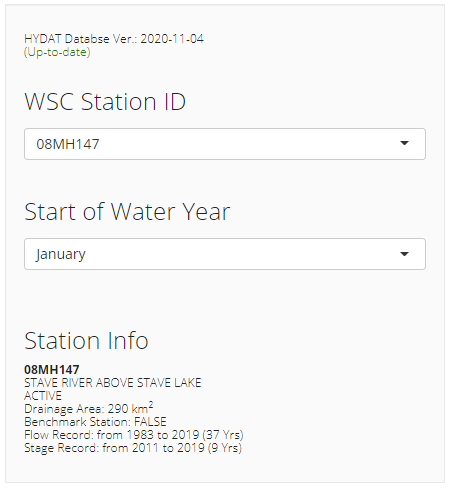

The app provides a brief description of the attributes of the station selected and will also determine if the HYDAT database used in the app is the latest available.

View the locations of WSC hydrometric stations in a simple (non-searchable) map. As shown on the figure below, clicking on a station location provides a summary of data available and station attributes.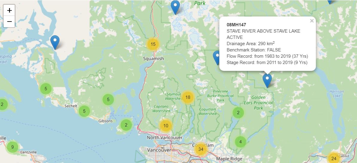

Select a hydrometric station and summarize streamflow data in a table format. Data can be summarized on a daily, monthly, or yearly basis and the summarized format can be downloaded as a csv file.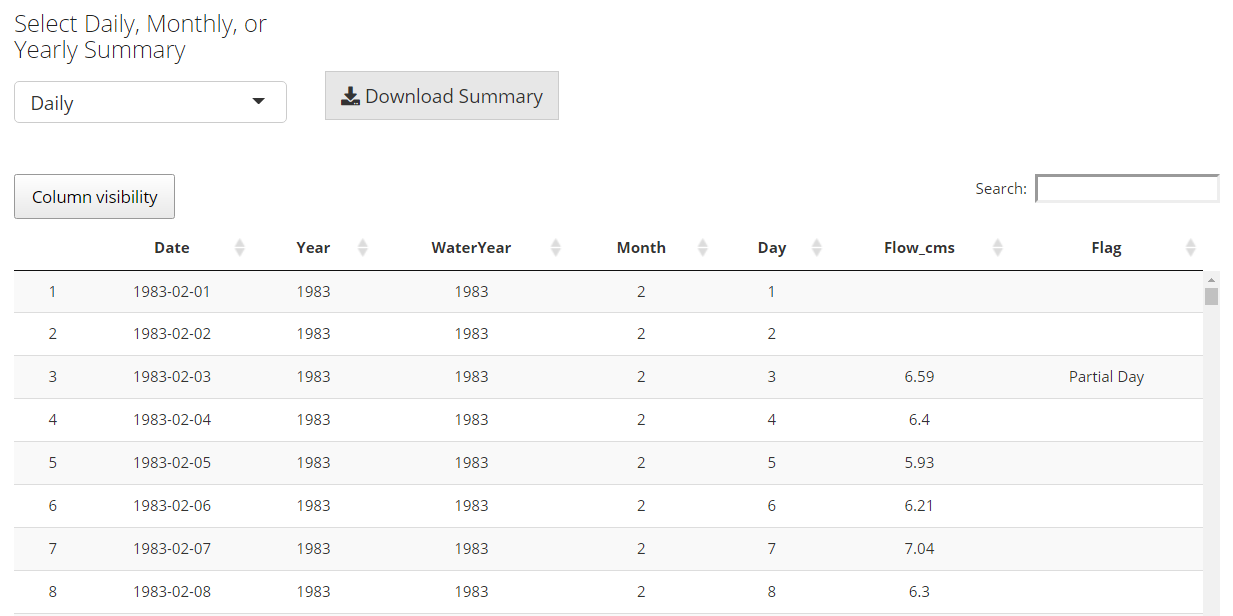

View the selected hydrometric station historical daily hydrograph in an interactive graph. The graph also displays data flags applicable to the record including estimated, partial days, ice conditions, dry, and revised. The purpose of this functionality is to allow a practitioner to quickly explore a station record without downloading data.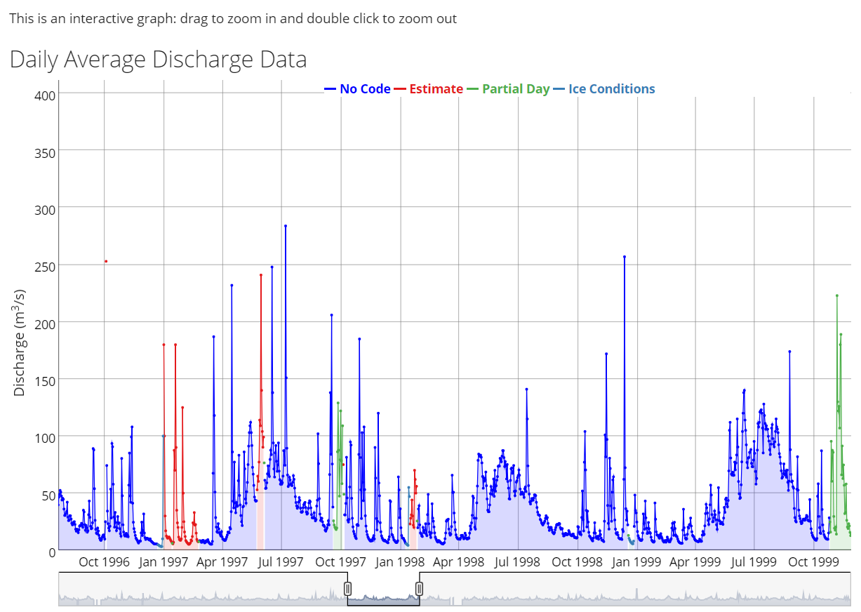

View the range of annual hydrograph data for the selected station. The graph displays the range of historical values for the annual hydrograph. This graph is generated using the FlowScreen package.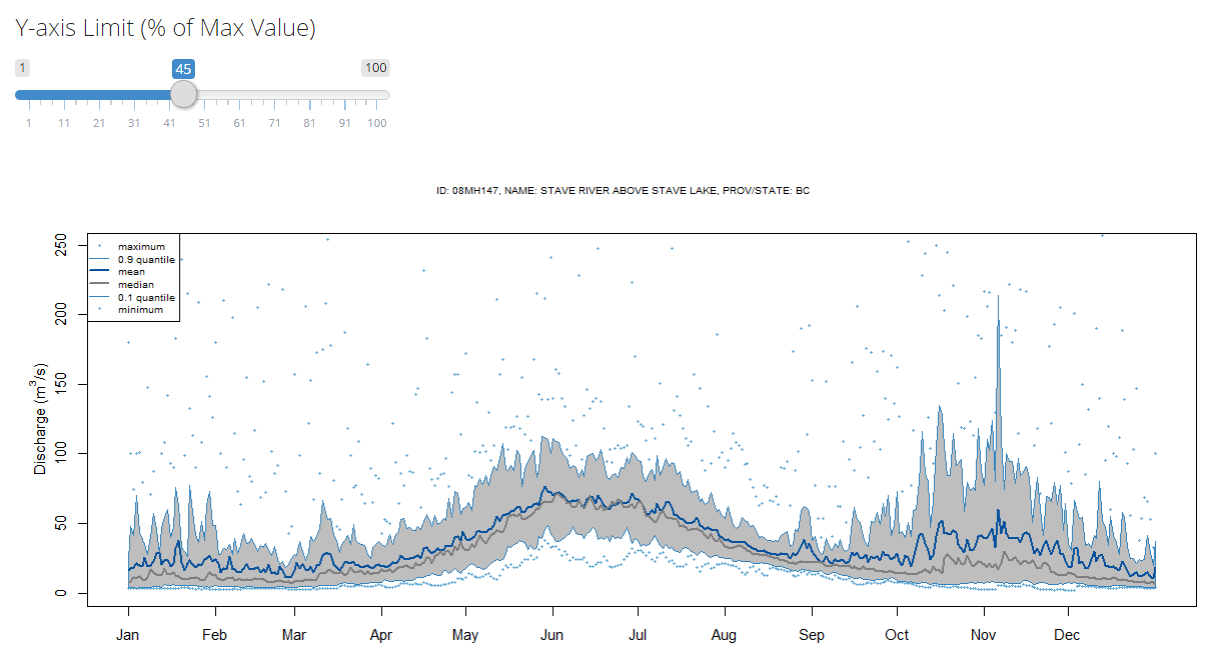

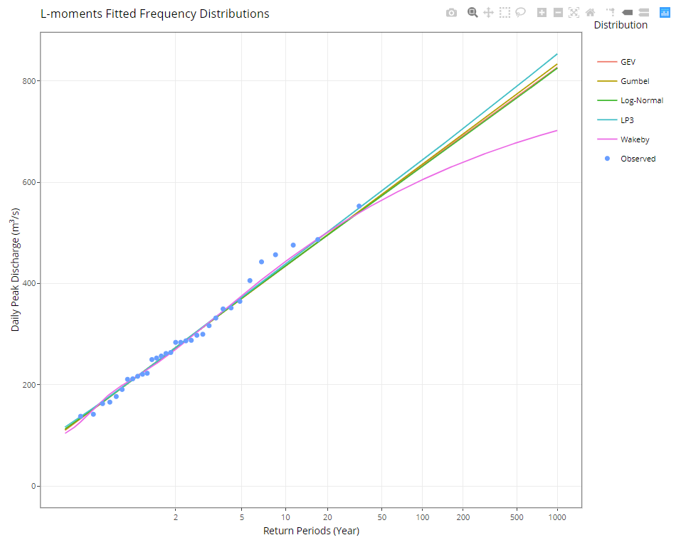
Run a flood frequency analysis (FFA) on the annual daily or instantaneous maximum streamflow series. A FFA computes return period estimates of flood events based on an observed record using extreme distributions (such as Log-Pearson III, Generalized Extreme Value (GEV), Gumbel, etc). The values of interest are typically beyond the period of record and result in extrapolations using the distributions. For example, one may be interested in estimating a 200-year return period daily flood event based on only 40 years of recorded streamflow data. Accordingly, there is usually a high amount of uncertainty associated with the estimated values.

To support the FFA analysis, the app functionality allows the user to customize the following:

• Remove specific years - the list of possible years to remove is auto-populated from the station record.
• Number of complete days per year - for example a user may want to exclude any years from the analysis containing less than 300 calendar days.
• The months to be considered in the analysis - in the event a user only wants to assess a specific season or an individual month.

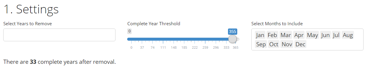
The record on which the FFA will be generated from is then provided in both table and graphical format for the user to review. Descriptive statistics based on the record are also provided.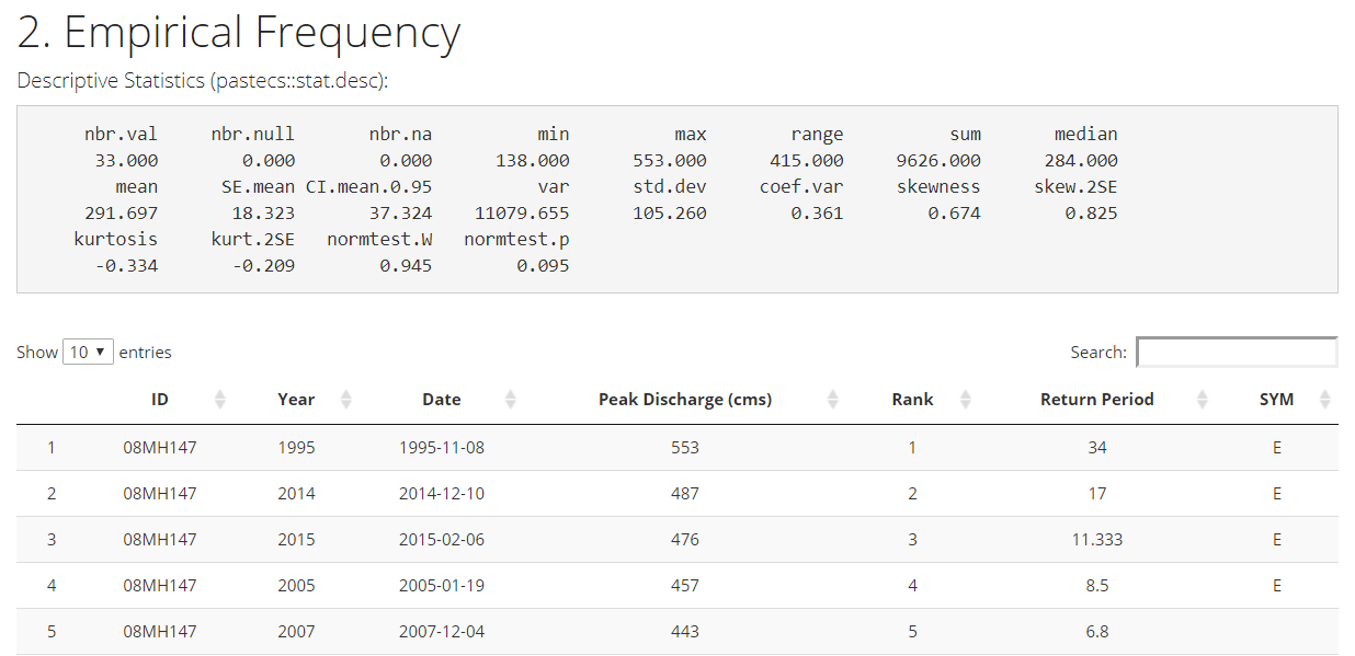

The user can then select the desired distribution used to fit the station record. The frequency distribution(s) are fitted using L-moments method from R package lmom by J. R. M. Hosking. L-moments of the sample data are calculated and distribution parameters are then estimated from the calculated L-moments. It is expected that a user completing a FFA through the app is sufficiently knowledgeable to perform the analysis and select appropriate distributions.

Further readings:

• Hosking, J., & Wallis, J. (1997). Regional Frequency Analysis: An Approach Based on L-Moments. Cambridge: Cambridge University Press. doi:10.1017/CBO9780511529443
• Makkonen, L. (2006). Plotting Positions in Extreme Value Analysis, Journal of Applied Meteorology and Climatology, 45(2), 334-340. doi:10.1175/JAM2349.1

The functionality is meant to provide an FFA exploratory tool giving a practitioner a better understanding of potential uncertainty in return period flood frequency estimates under various distributions or periods of record.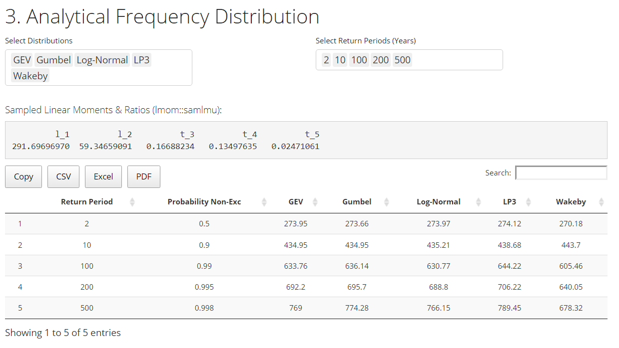

In general, the FFA capability of the app is considered as an ‘advanced’ feature to support practitioners with knowledge in this area. However, the streamflow record exploratory functionality should still be provide other users of the app with value.

It should also be recognized that there are packages that provide more streamflow exploration and FFA capability than are available through this app. In particular, the CSHShydRology package in R is under ongoing development by the Canadian Society for Hydrological Sciences and may be of interest to practitioners looking for more in depth functionality (currently with no application interface).

Hosting the Application

The app was originally completed with the purpose of learning Shiny and the intent was that the app could be hosted locally from RStudio to support data exploration if useful. An attempt was originally made to host the app on the free tier of shinyapps.io but the performance of the app was extremely slow (likely due to the size of the database and the large number of packages required).

Recently, an additional attempt was made to deploy the application on shinyapps.io with the step of removing data not used by the application from the SQLite database. The hope was that the reduced SQLite database would improve the app performance. However, while faster than the original attempt, the performance was still not adequate and led to building a Shiny Server on an EC2 instance in AWS. Trying to deploy an app from a cloud service was a new experience and I was fortunately able to find the following guide by Charles Bordet which steps through the process: https://www.charlesbordet.com/en/guide-shiny-aws/. There were a couple of snags but overall the instructions were very good resulting in successful deployment.

Note: The app is currently hosted on shinyapps.io lowest paid tier which is slightly cheaper than AWS and can be found here.

Project Lessons

The ShinyCFA application was approached with a learning objective and ended up as a useful project for that purpose including:

Learning how to create a Shiny application: This was the original objective of the project and was successful. However, looking back at the code there are also lessons learned including:

• Scope creep: The app we originally set out to build had a smaller scope, and as we were building more functionality was added. This led to a less than ideal organization of code which is not very modularized. Recently, a few minor fixes to the app ended up being more complicated than anticipated.
• Shiny reactivity: We were learning on an as needed basis while building the app and it isn’t optimized in terms of reactivity. We have found working on subsequent projects that app performance can certainly be improved by paying attention to this.
• General coding style: If one had to go back and make large modifications to the application it would not be easy.

Collaborative Development: Prior to this project Nick and I had not worked collaboratively on code and this was a good opportunity to learn in this area. In hindsight our collaborative approach lacked important aspects such as code reviews on PRs but it was a good first attempt.

Deploying Applications: While this wasn’t an initial goal of the project it ended up working as a useful test app for hosting a cloud based application. Hosting on AWS likely wouldn’t have been pursued if the performance of the application was adequate on shinyapps.io. This requires more learning such as cloud security and looking at the use of additional AWS tools, but was a good opportunity to dive into this area.

While the application likely won’t be used for future development in preference of working with different datasets, it was considered a success for the learning objectives it supported.